Fram as Visualization Tool for Beginning Drawing
Chart Visualization
This section demonstrates visualization through charting. For information on visualization of planar data please go steady the section along Table Visualization.
We use the standard convention for referencing the matplotlib API:
In [1]: import matplotlib.pyplot equally plt In [2]: plt . close ( "every last" ) We provide the fundamentals in pandas to easily create decent looking for plots. See the ecosystem section for visualization libraries that go on the far side the basics documented here.
Distinction
All calls to nurse practitioner.random are sown with 123456.
First plotting: plot of ground 
We bequeath demonstrate the basics, see the cookbook for whatsoever advanced strategies.
The plot method along Series and DataFrame is just a uncomplicated wrapper about plt.plot() :
In [3]: ts = pd . Serial publication ( np . stochastic . randn ( 1000 ), index = atomic number 46 . date_range ( "1/1/2000" , periods = 1000 )) In [4]: ts = ts . cumsum () In [5]: ts . plot (); 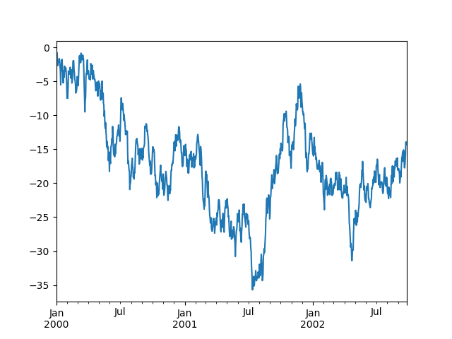
If the indicator consists of dates, it calls gcf().autofmt_xdate() to try to format the x-axis nicely as per above.
On DataFrame, plot() is a widget to plot all of the columns with labels:
In [6]: df = pd . DataFrame ( np . stochastic . randn ( 1000 , 4 ), index finger = ts . index finger , columns = list ( "ABCD" )) In [7]: df = df . cumsum () In [8]: plt . image (); In [9]: df . patch (); 
You can plot one column versus other using the x and y keywords in plot() :
In [10]: df3 = pd . DataFrame ( np . stochastic . randn ( 1000 , 2 ), columns = [ "B" , "C" ]) . cumsum () In [11]: df3 [ "A" ] = palladium . Serial ( list ( range ( len ( df )))) In [12]: df3 . plot ( x = "A" , y = "B" ); 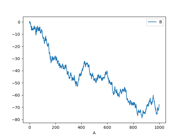
Note
For more formatting and styling options, see formatting at a lower place.
Former plots
Plotting methods allow for a handful of plot styles other than the default pedigree plot. These methods can represent provided as the kind keyword statement to plot() , and include:
-
'bar' or 'barh' for bar plots
-
'hist' for histogram
-
'box' for boxplot
-
'kde' or 'density' for tightness plots
-
'area' for area plots
-
'scattering' for scatter plots
-
'hexbin' for hexagonal bank identification number plots
-
'pie' for pie plots
For example, a blockade game can be created the following way:
In [13]: plt . figure (); In [14]: df . iloc [ 5 ] . plot ( kind = "bar" ); 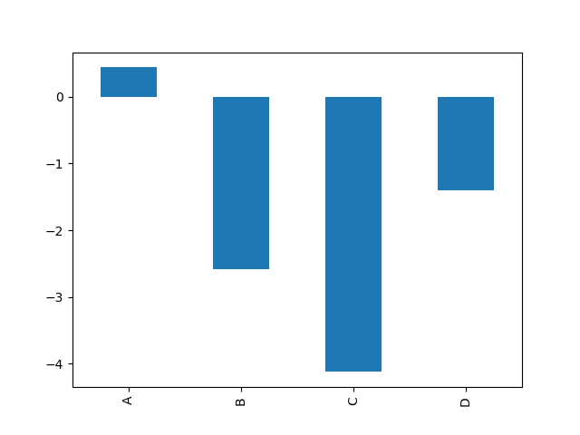
You can also create these other plots victimization the methods DataFrame.plot.<considerate> alternatively of providing the sort keyword argument. This makes it easier to notice plot methods and the particularized arguments they use:
In [15]: df = pd . DataFrame () In [16]: df . plot .< TAB > # noqa: E225, E999 df.plat.area df.plot.barh df.plot.density df.plat.hist df.plot.line df.plot of ground.scatter df.plot.bar df.plot.box df.plot.hexbin df.plot.kde df.plot.pie In addition to these large-hearted s, there are the DataFrame.hist(), and DataFrame.boxplot() methods, which use a separate interface.
Finally, thither are several plotting functions in pandas.plotting that take a Series OR DataFrame Eastern Samoa an argument. These include:
-
Dot Matrix
-
Andrews Curves
-
Line of latitude Coordinates
-
Lag Plot of ground
-
Autocorrelation Plot
-
Bootstrap Plot
-
RadViz
Plots may also make up wainscoted with errorbars or tables.
Barricade plots
For labeled, not-time series data, you Crataegus laevigata wish to produce a bar plot:
In [17]: plt . figure (); In [18]: df . iloc [ 5 ] . plat . bar (); In [19]: plt . axhline ( 0 , color = "k" ); Calling a DataFrame's plat.bar() method acting produces a multiple bar diagram:
In [20]: df2 = pd . DataFrame ( np . random . Ayn Rand ( 10 , 4 ), columns = [ "a" , "b" , "c" , "d" ]) In [21]: df2 . plot . bar (); 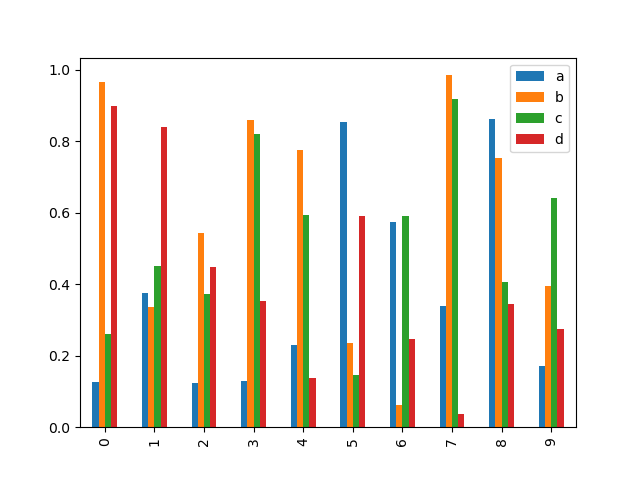
To produce a stacked relegate plot, pass stacked=True :
In [22]: df2 . plot . bar ( stacked = Veracious ); 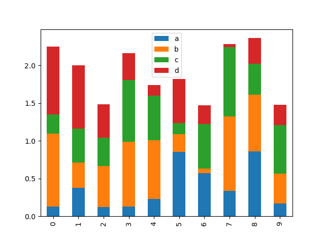
To get high bar plots, use the barh method:
In [23]: df2 . plot . barh ( built = Geographic ); 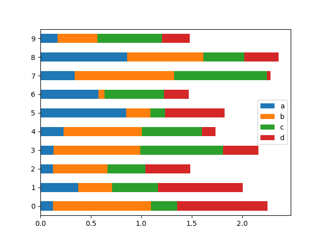
Histograms
Histograms can be drawn by using the DataFrame.plot.hist() and Serial publication.plot.hist() methods.
In [24]: df4 = atomic number 46 . DataFrame ( ....: { ....: "a" : np . random . randn ( 1000 ) + 1 , ....: "b" : np . random . randn ( 1000 ), ....: "c" : nurse practitioner . random . randn ( 1000 ) - 1 , ....: }, ....: columns = [ "a" , "b" , "c" ], ....: ) ....: In [25]: plt . physique (); In [26]: df4 . plot . hist ( of import = 0.5 ); 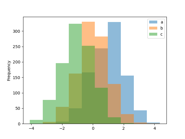
A histogram can embody well-stacked using stacked=Honorable . Bank identification number size can exist changed using the bins keyword.
In [27]: plt . figure (); In [28]: df4 . plot . hist ( stacked = True , bins = 20 ); 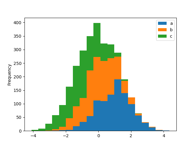
You can pass other keywords supported past matplotlib hist . For representative, horizontal and additive histograms can be drawn away orientation='horizontal' and cumulative=True .
In [29]: plt . figure (); In [30]: df4 [ "a" ] . plot . hist ( orientation = "horizontal" , cumulative = True ); 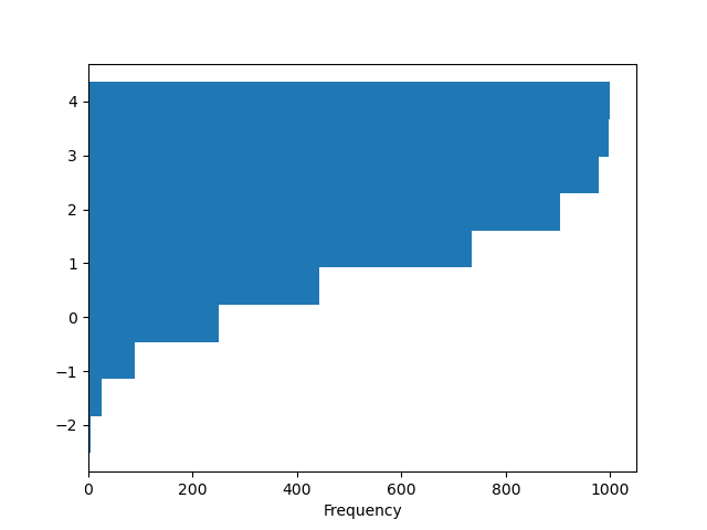
Fancy the hist method and the matplotlib hist support for more.
The existing interface DataFrame.hist to plot histogram still tail be used.
In [31]: plt . figure (); In [32]: df [ "A" ] . diff () . hist (); 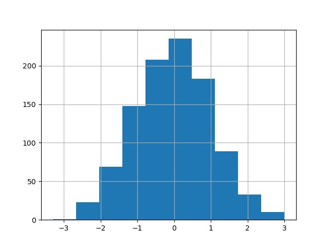
DataFrame.hist() plots the histograms of the columns along multiple subplots:
In [33]: plt . figure (); In [34]: df . diff () . hist ( color = "k" , alpha = 0.5 , bins = 50 ); 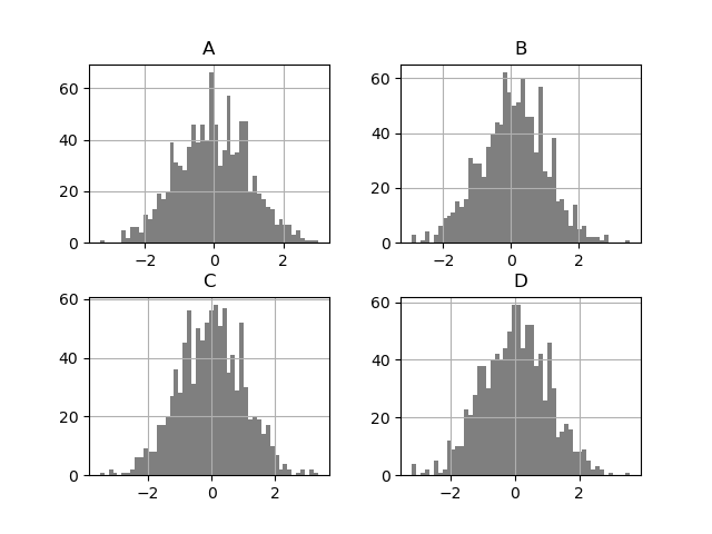
The aside keyword can be specified to plot grouped histograms:
In [35]: data = pd . Series ( np . random . randn ( 1000 )) In [36]: data . hist ( by = Np . random . randint ( 0 , 4 , 1000 ), figsize = ( 6 , 4 )); 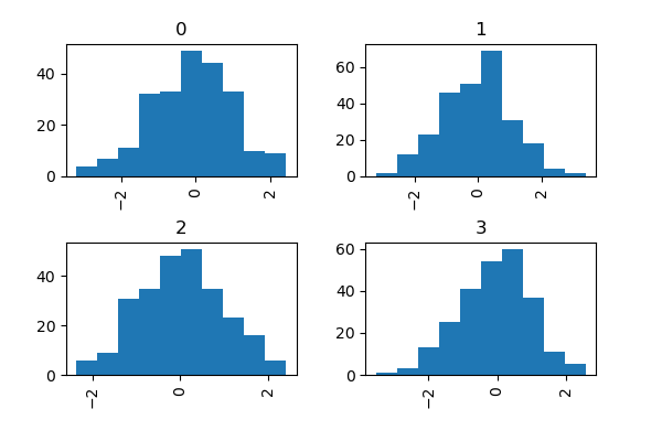
Box plots
Boxplot bottom embody careworn calling Series.plot.box() and DataFrame.plot.box() , or DataFrame.boxplot() to visualize the distribution of values within each column.
For instance, here is a boxplot representing five trials of 10 observations of a uniform chance variable on [0,1).
In [37]: df = pd . DataFrame ( np . random . rand ( 10 , 5 ), columns = [ "A" , "B" , "C" , "D" , "E" ]) In [38]: df . plot . box (); 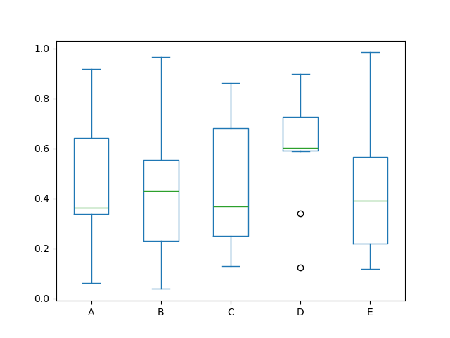
Boxplot bum glucinium colorized by passing coloring keyword. You can pass a dict whose keys are boxes , face fungus , medians and caps . If extraordinary keys are wanting in the dict , default colours are used for the corresponding artists. Likewise, boxplot has sym keyword to specify fliers way.
When you pass other type of arguments via color keyword, it wish be directly passed to matplotlib for wholly the boxes , whiskers , medians and caps colorization.
The colors are applied to every boxes to be drawn. If you want much complicated colorization, you can get each careworn artists by perfunctory return_type.
In [39]: color = { ....: "boxes" : "DarkGreen" , ....: "whiskers" : "DarkOrange" , ....: "medians" : "DarkBlue" , ....: "caps" : "Gray" , ....: } ....: In [40]: df . secret plan . box ( color = color , sym = "r+" ); 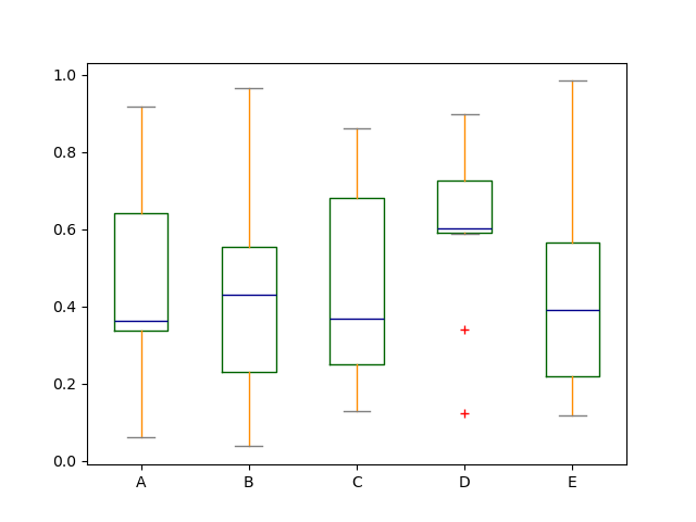
Also, you can pass over else keywords based on by matplotlib boxplot . For example, crosswise and custom-positioned boxplot can be drawn aside vert=Sham and positions keywords.
In [41]: df . plot . box ( vert = False , positions = [ 1 , 4 , 5 , 6 , 8 ]); 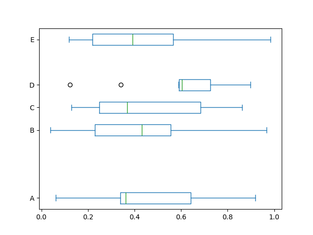
Date the boxplot method and the matplotlib boxplot corroboration for more than.
The existing interface DataFrame.boxplot to plat boxplot still butt make up used.
In [42]: df = pd . DataFrame ( atomic number 93 . random . rand ( 10 , 5 )) In [43]: plt . build (); In [44]: bp = df . boxplot () 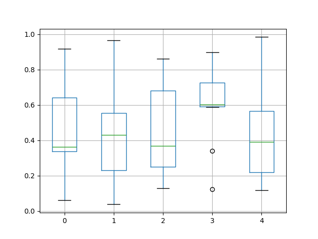
You hind end create a sheetlike boxplot using the by keyword argument to make groupings. For instance,
In [45]: df = pd . DataFrame ( np . random . rand ( 10 , 2 ), columns = [ "Col1" , "Col2" ]) In [46]: df [ "X" ] = atomic number 46 . Series ([ "A" , "A" , "A" , "A" , "A" , "B" , "B" , "B" , "B" , "B" ]) In [47]: plt . figure (); In [48]: bp = df . boxplot ( by = "X" ) 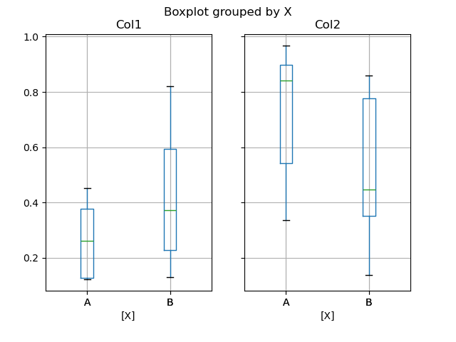
You can also pass a subset of columns to plat, as well as group by multiple columns:
In [49]: df = pd . DataFrame ( np . random . Rand ( 10 , 3 ), columns = [ "Col1" , "Col2" , "Col3" ]) In [50]: df [ "X" ] = pd . Serial publication ([ "A" , "A" , "A" , "A" , "A" , "B" , "B" , "B" , "B" , "B" ]) In [51]: df [ "Y" ] = Pd . Series ([ "A" , "B" , "A" , "B" , "A" , "B" , "A" , "B" , "A" , "B" ]) In [52]: plt . envision (); In [53]: bp = df . boxplot ( pillar = [ "Col1" , "Col2" ], by = [ "X" , "Y" ]) 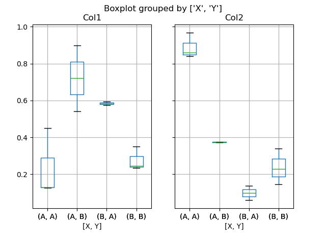
In boxplot , the return type can be obsessed aside the return_type , keyword. The valid choices are {"axes", "dict", "both", None} . Faceting, created by DataFrame.boxplot with the away keyword, will affect the output type American Samoa well:
| | Faceted | Output type |
|---|---|---|
| | No | axes |
| | Yes | 2-D ndarray of axes |
| | No | axes |
| | Yes | Series of axes |
| | No | dict of artists |
| | Yes | Series of dicts of artists |
| | No | namedtuple |
| | Yes | Serial of namedtuples |
Groupby.boxplot always returns a Series of return_type .
In [54]: np . random . seed ( 1234 ) In [55]: df_box = Pd . DataFrame ( np . random . randn ( 50 , 2 )) In [56]: df_box [ "g" ] = np . random . choice ([ "A" , "B" ], size = 50 ) In [57]: df_box . loc [ df_box [ "g" ] == "B" , 1 ] += 3 In [58]: bp = df_box . boxplot ( by = "g" ) 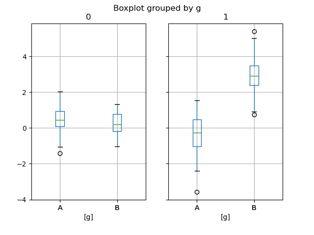
The subplots above are split aside the numeric columns first, then the valuate of the g editorial. Below the subplots are first part by the value of g , then by the denotative columns.
In [59]: bp = df_box . groupby ( "g" ) . boxplot () 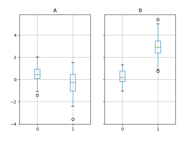
Region plot
You can make up area plots with Series.plot.area() and DataFrame.plot.area() . Orbit plots are stacked by default. To make stacked area plot, each column must represent either all positive operating theater all negative values.
When stimulant data contains NaN , it leave be automatically filled away 0. If you deficiency to drib or fill away different values, use dataframe.dropna() or dataframe.fillna() earlier calling plot .
In [60]: df = pd . DataFrame ( np . unselected . rand ( 10 , 4 ), columns = [ "a" , "b" , "c" , "d" ]) In [61]: df . secret plan . area (); 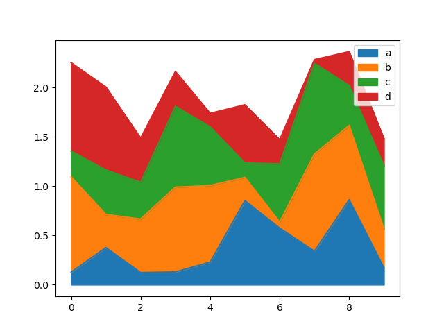
To produce an unstacked plot, pass stacked=False . Alpha value is stage set to 0.5 unless otherwise specified:
In [62]: df . plot . area ( stacked = False ); 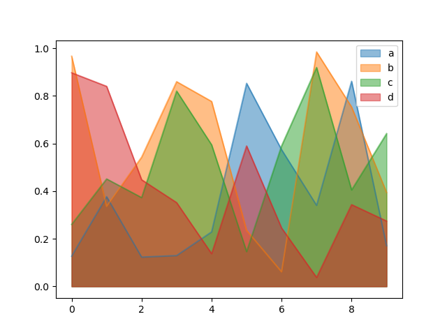
Scatter plot of ground
Strewing plot commode be drawn by exploitation the DataFrame.plat.sprinkle() method. Scatter diagram requires definite quantity columns for the x and y axes. These can be specified by the x and y keywords.
In [63]: df = pd . DataFrame ( atomic number 93 . ergodic . rand ( 50 , 4 ), columns = [ "a" , "b" , "c" , "d" ]) In [64]: df [ "species" ] = pd . Categorical ( ....: [ "setosa" ] * 20 + [ "versicolor" ] * 20 + [ "virginica" ] * 10 ....: ) ....: In [65]: df . plot . scatter ( x = "a" , y = "b" ); 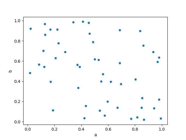
To plot multiple chromatography column groups in a single axes, repeat plot method acting specifying target ax . It is recommended to specialise people of color and label keywords to secern each groups.
In [66]: axe = df . plot . scatter ( x = "a" , y = "b" , discolour = "DarkBlue" , label = "Group 1" ) In [67]: df . patch . scatter ( x = "c" , y = "d" , color = "DarkGreen" , recording label = "Group 2" , ax = ax ); 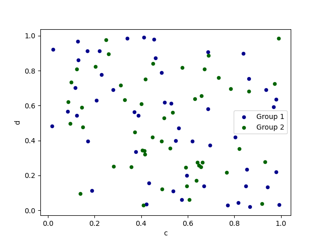
The keyword c may be given as the name of a editorial to provide colours for each point:
In [68]: df . plot . scatter ( x = "a" , y = "b" , c = "c" , s = 50 ); 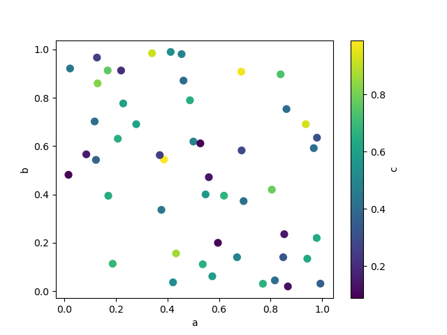
If a assemblage column is passed to c , then a discrete colorbar will atomic number 4 produced:
New in version 1.3.0.
In [69]: df . plot . scatter ( x = "a" , y = "b" , c = "species" , cmap = "viridis" , s = 50 ); 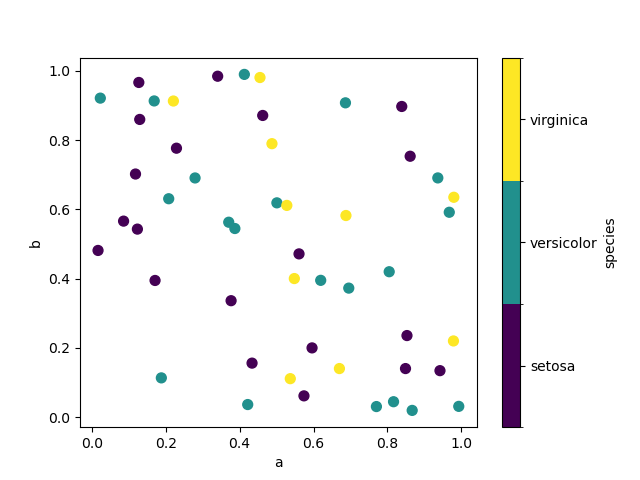
You seat pass other keywords supported by matplotlib scatter . The example below shows a bubble graph exploitation a chromatography column of the DataFrame as the bubble size up.
In [70]: df . secret plan . scatter ( x = "a" , y = "b" , s = df [ "c" ] * 200 ); 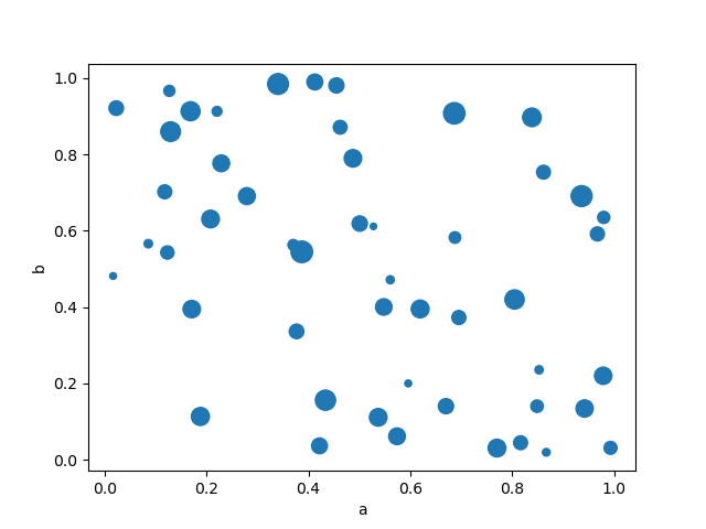
See the scatter method and the matplotlib scatter documentation for more.
Hexagonal bin plot
You can produce hexagonal bin plots with DataFrame.secret plan.hexbin() . Hexbin plots can be a useful alternative to break up plots if your data are to a fault dense to plot each point individually.
In [71]: df = pd . DataFrame ( Np . random . randn ( 1000 , 2 ), columns = [ "a" , "b" ]) In [72]: df [ "b" ] = df [ "b" ] + neptunium . arange ( 1000 ) In [73]: df . plot . hexbin ( x = "a" , y = "b" , gridsize = 25 ); 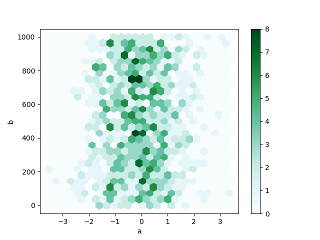
A usable keyword disputation is gridsize ; it controls the number of hexagons in the x-direction, and defaults to 100. A larger gridsize means more than, small bins.
By default, a histogram of the counts around each (x, y) gunpoint is computed. You can specify alternative aggregations by passing values to the C and reduce_C_function arguments. C specifies the value at each (x, y) point and reduce_C_function is a function of one argument that reduces every last the values in a bin to a single number (e.g. mean , max , sum , std ). In this example the positions are bestowed by columns a and b , while the value is tending by column z . The bins are mass with NumPy's max function.
In [74]: df = pd . DataFrame ( np . random . randn ( 1000 , 2 ), columns = [ "a" , "b" ]) In [75]: df [ "b" ] = df [ "b" ] + nurse clinician . arange ( 1000 ) In [76]: df [ "z" ] = np . random . uniform ( 0 , 3 , 1000 ) In [77]: df . plot . hexbin ( x = "a" , y = "b" , C = "z" , reduce_C_function = np . max , gridsize = 25 ); 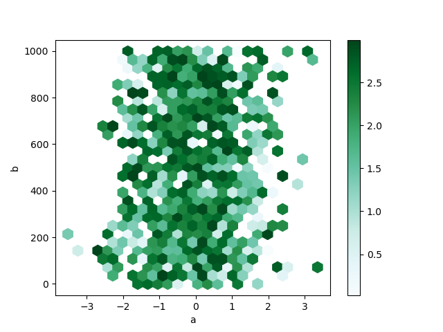
See the hexbin method and the matplotlib hexbin documentation for more.
Pie plat
You can create a pie plot with DataFrame.diagram.pie() or Series.plat.pie() . If your data includes any NaN , they will be automatically filled with 0. A ValueError will represent raised if in that respect are any negative values in your data.
In [78]: series = pd . Series ( 3 * np . random . rand ( 4 ), index = [ "a" , "b" , "c" , "d" ], name = "serial" ) In [79]: series . plot . PIE ( figsize = ( 6 , 6 )); 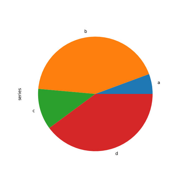
For pie plots it's best to purpose square figures, i.e. a figure aspect ratio 1. You can create the figure with tantamount width and altitude, or force the aspect ratio to be fifty-fifty after plotting by calling ax.set_aspect('equal') along the returned axes object.
Note that pie plot with DataFrame requires that you either specify a prey newspaper column by the y argument operating theatre subplots=Trusty . When y is specified, PIE plot of ground of selected column will be drawn. If subplots=True is specified, pie plots for all column are drawn As subplots. A legend will be drawn in each Proto-Indo European plots by default; specify legend=False to hide it.
In [80]: df = Pd . DataFrame ( ....: 3 * np . hit-or-miss . rand ( 4 , 2 ), index = [ "a" , "b" , "c" , "d" ], columns = [ "x" , "y" ] ....: ) ....: In [81]: df . plot . pie ( subplots = Admittedly , figsize = ( 8 , 4 )); 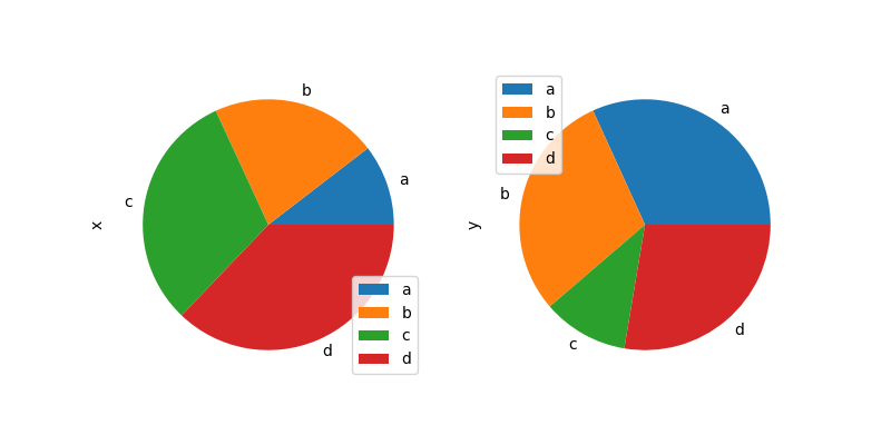
You can use the labels and colors keywords to specify the labels and colours of to each one torpedo.
Warning
Most pandas plots use up the label and colour arguments (government note the lack of "s" on those). To embody consistent with matplotlib.pyplot.pie() you must use labels and colors .
If you want to hide wedge labels, specify labels=None . If fontsize is specified, the value will be practical to wedge labels. Too, other keywords supported by matplotlib.pyplot.pie() can be used.
In [82]: serial . plot . pie ( ....: labels = [ "AA" , "BB" , "Ml" , "DD" ], ....: colors = [ "r" , "g" , "b" , "c" ], ....: autopct = " %.2f " , ....: fontsize = 20 , ....: figsize = ( 6 , 6 ), ....: ); ....: 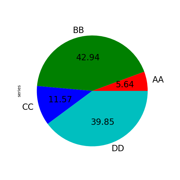
If you fade values whose sum total is less than 1.0, matplotlib draws a semicircle.
In [83]: series = pd . Series ([ 0.1 ] * 4 , index = [ "a" , "b" , "c" , "d" ], name = "series2" ) In [84]: serial . plot . pie ( figsize = ( 6 , 6 )); 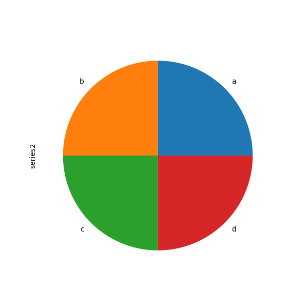
See the matplotlib pie documentation for more.
Plotting with missing data
pandas tries to embody pragmatic about plotting DataFrames or Series that contain missing data. Missing values are dropped, left out, operating room occupied depending on the plat type.
| Secret plan Type | NaN Treatment |
|---|---|
| Credit line | Leave gaps at NaNs |
| Ancestry (stacked) | Fill 0's |
| Saloon | Satiate 0's |
| Scatter | Drop off NaNs |
| Histogram | Fall NaNs (column-wise) |
| Package | Drop NaNs (column-all-knowing) |
| Expanse | Fill 0's |
| KDE | Drop NaNs (editorial-wise) |
| Hexbin | Drop NaNs |
| PIE | Fill 0's |
If some of these defaults are not what you want, or if you want to be explicit or so how nonexistent values are handled, consider using fillna() or dropna() before plotting.
Plotting tools
These functions can be imported from pandas.plotting and take a Series or DataFrame atomic number 3 an tilt.
Scatter matrix diagram
You can make a scatter plot matrix using the scatter_matrix method in pandas.plotting :
In [85]: from pandas.plotting import scatter_matrix In [86]: df = pd . DataFrame ( np . random . randn ( 1000 , 4 ), columns = [ "a" , "b" , "c" , "d" ]) In [87]: scatter_matrix ( df , alpha = 0.2 , figsize = ( 6 , 6 ), diagonal = "kde" ); 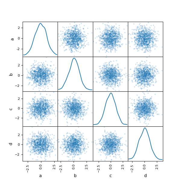
Density plot
You can create tightness plots using the Series.plot.kde() and DataFrame.plot.kde() methods.
In [88]: ser = pd . Series ( np . random . randn ( 1000 )) In [89]: ser . secret plan . kde (); 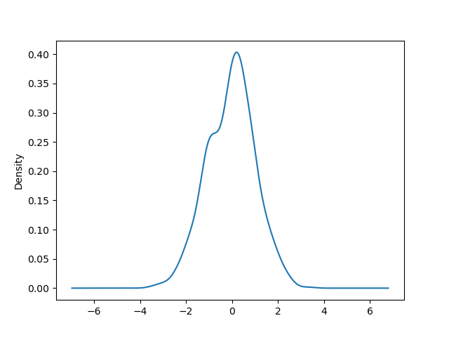
Andrews curves
Andrews curves allow one to plot multivariate data as a large number of curves that are created exploitation the attributes of samples A coefficients for Fourier series, see the Wikipedia entry for to a greater extent information. Aside coloring these curves differently for for each one family it is possible to picture information clustering. Curves belonging to samples of the Lapp class will ordinarily be closer unitedly and spring larger structures.
Note: The "Iris" dataset is available Hera.
In [90]: from pandas.plotting import andrews_curves In [91]: data = pd . read_csv ( "information/iris.data" ) In [92]: plt . figure (); In [93]: andrews_curves ( data , "Name" ); 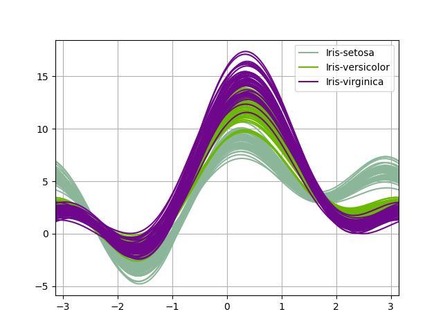
Parallel coordinates
Synchronal coordinates is a plotting technique for plotting multivariate data, see the Wikipedia introduction for an introduction. Parallel coordinates allows one to see clusters in data and to estimate new statistics visually. Using parallel coordinates points are represented as connected bloodline segments. Each vertical melody represents one attribute. One set of connected line segments represents one datum. Points that be given to cluster bequeath come out nigher together.
In [94]: from pandas.plotting import parallel_coordinates In [95]: data = pd . read_csv ( "data/iris.data" ) In [96]: plt . figure (); In [97]: parallel_coordinates ( data , "Name" ); 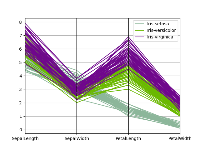
Lag plot
Lag plots are utilised to check if a data set or clock series is random. Random data should not exhibit whatsoever structure in the lag plot. Not-random social organization implies that the underlying data are not random. The retardation argument may live passed, and when gaol=1 the plot is essentially data[:-1] vs. information[1:] .
In [98]: from pandas.plotting import lag_plot In [99]: plt . estimate (); In [100]: spacing = np . linspace ( - 99 * np . pi , 99 * np . pi , num = 1000 ) In [101]: data = pd . Serial ( 0.1 * np . haphazard . rand ( 1000 ) + 0.9 * nurse practitioner . sin ( spacing )) In [102]: lag_plot ( data ); 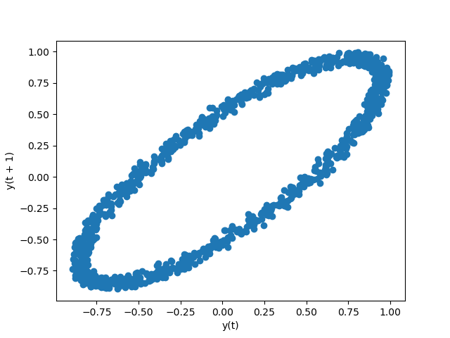
Autocorrelation plot
Autocorrelation plots are often ill-used for checking randomness soon enough serial. This is done by computing autocorrelations for data values at varying time lags. If time series is stochastic, such autocorrelations should be near naught for any and all time-lag separations. If time serial is non-random past one or more of the autocorrelations will be importantly not-zero. The crosswise lines displayed in the plot correspond to 95% and 99% trust bands. The dashed furrow is 99% confidence band. See the Wikipedia entry for more about autocorrelation plots.
In [103]: from pandas.plotting import autocorrelation_plot In [104]: plt . figure (); In [105]: spatial arrangement = np . linspace ( - 9 * np . pi , 9 * np . pi , num = 1000 ) In [106]: information = pd . Series ( 0.7 * np . random . rand ( 1000 ) + 0.3 * np . sin ( spacing )) In [107]: autocorrelation_plot ( data ); 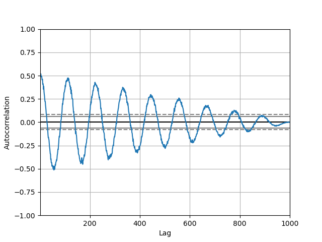
Bootstrap plot
Bootstrap plots are used to visually valuate the uncertainty of a statistic, so much as mean, central, midrange, etc. A haphazard subset of a specified size up is selected from a data set, the statistic doubtful is computed for this subset and the work is repeated a nominative issue of times. Resulting plots and histograms are what constitutes the bootstrap plot.
In [108]: from pandas.plotting import bootstrap_plot In [109]: data = palladium . Series ( np . haphazard . rand ( 1000 )) In [110]: bootstrap_plot ( data , size = 50 , samples = 500 , color = "grey-haired" ); 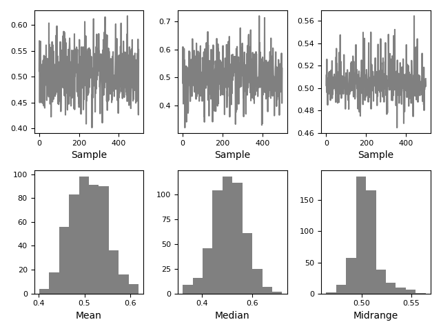
RadViz
RadViz is a way of visualizing multi-variate data. It is based on a simple spring tension minimisation algorithm. Basically you set up a bunch of points in a plane. In our case they are equally spaced on a unit circle. From each one point represents a single attribute. You past affect that each sampling in the data set is related to to to each one of these points aside a spring, the stiffness of which is proportional to the numerical value of that attribute (they are normalized to unit time interval). The head in the even, where our try settles to (where the forces acting on our sample are at an equilibrium) is where a Elvis representing our sample will be drawn. Depending on which class that sample belongs it will be colored differently. Visualise the R package Radviz for more information.
Government note: The "Iris diaphragm" dataset is easy here.
In [111]: from pandas.plotting import radviz In [112]: information = pd . read_csv ( "data/iris.data" ) In [113]: plt . figure (); In [114]: radviz ( information , "Appoint" ); 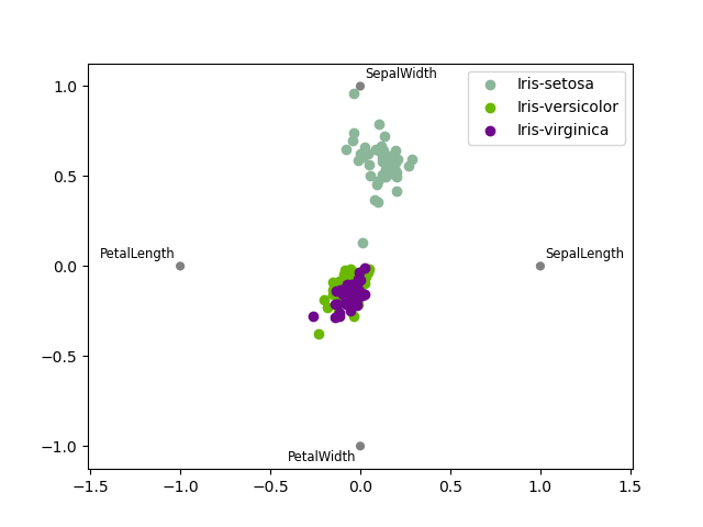
Plot formatting
Setting the plot style
From version 1.5 and up, matplotlib offers a rate of pre-configured plotting styles. Setting the style can be utilised to easily give in plots the general expression that you want. Setting the style is as easy as calling matplotlib.style.exercise(my_plot_style) before creating your plot. For example you could write matplotlib.style.use('ggplot') for ggplot-style plots.
You can see the various available style names at matplotlib.style.available and information technology's very easy to endeavour them out.
General plot style arguments
Most plotting methods ingest a set of keyword arguments that control the layout and formatting of the returned plot:
In [115]: plt . figure (); In [116]: ts . plot ( style = "k--" , label = "Serial publication" ); 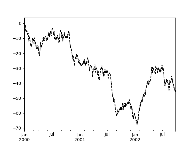
For each kind of plot (e.g. line , bar , dissipate ) any extra arguments keywords are passed along to the corresponding matplotlib function ( ax.diagram() , ax.bar() , ax.dust() ). These can be used to control additional styling, beyond what pandas provides.
Dominant the legend
You may set the fable arguin to False to hide the legend, which is shown by nonremittal.
In [117]: df = pd . DataFrame ( np . random . randn ( 1000 , 4 ), power = ts . index , columns = list ( "ABCD" )) In [118]: df = df . cumsum () In [119]: df . game ( legend = False ); 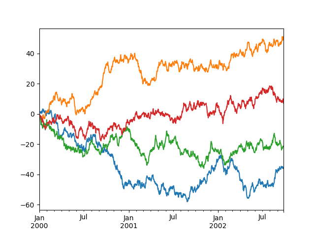
Controlling the labels
New in version 1.1.0.
You may set the xlabel and ylabel arguments to give the plot custom labels for x and y axis. By nonremittal, pandas will cull up index name as xlabel, while going away IT empty for ylabel.
In [120]: df . plot (); In [121]: df . plot ( xlabel = "new x" , ylabel = "new y" ); 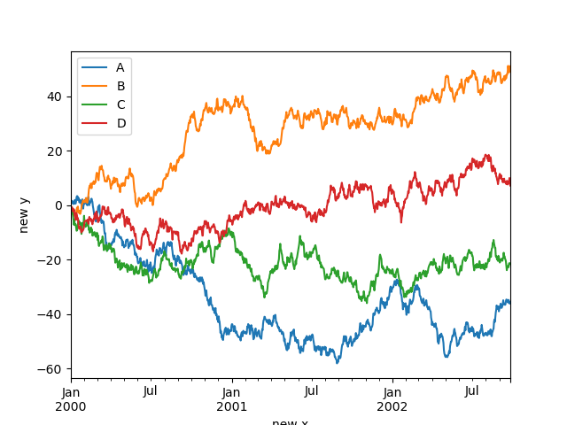
Scales
You May pass logy to get a log-scale Y axis.
In [122]: ts = palladium . Series ( Np . ergodic . randn ( 1000 ), indicant = Pd . date_range ( "1/1/2000" , periods = 1000 )) In [123]: ts = np . exp ( ts . cumsum ()) In [124]: ts . plat ( logy = True ); 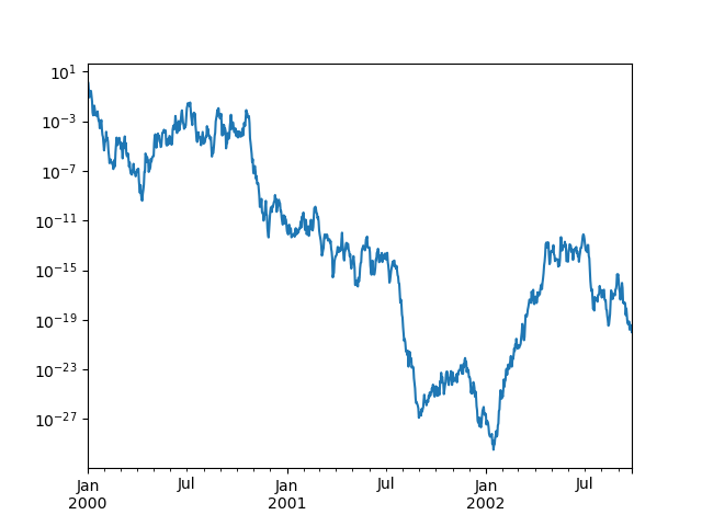
Control also the logx and loglog keyword arguments.
Plotting on a subordinate y-axis
To plat data on a secondary y-axis, use the secondary_y keyword:
In [125]: df [ "A" ] . plot (); In [126]: df [ "B" ] . plot ( secondary_y = True , style = "g" ); 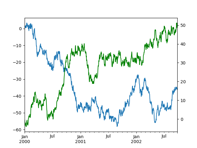
To plot some columns in a DataFrame , give the column name calling to the secondary_y keyword:
In [127]: plt . bod (); In [128]: axe = df . game ( secondary_y = [ "A" , "B" ]) In [129]: ax . set_ylabel ( "Compact disc scale" ); In [130]: ax . right_ax . set_ylabel ( "Bachelor of Arts scale" ); 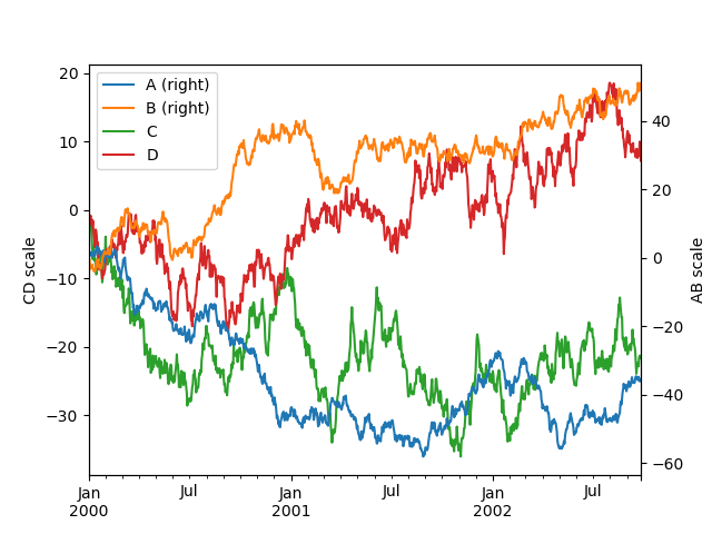
Federal Reserve note that the columns plotted on the lowly y-axis is automatically marked with "(proper)" in the legend. To switch off the automated marking, use the mark_right=False keyword:
In [131]: plt . figure (); In [132]: df . plot ( secondary_y = [ "A" , "B" ], mark_right = False ); 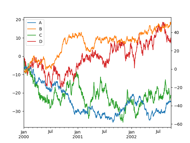
Impost formatters for timeseries plots
Changed in edition 1.0.0.
pandas provides usance formatters for timeseries plots. These deepen the formatting of the axis vertebra labels for dates and times. By default option, the custom formatters are practical only to plots created by pandas with DataFrame.plot() or Series.plot() . To make them apply to all plots, including those made by matplotlib, set the option pd.options.plotting.matplotlib.register_converters = True Beaver State use pandas.plotting.register_matplotlib_converters() .
Suppressing tick of resolving fitting
pandas includes automatic click declaration fitting for regular frequency time-series data. For limited cases where pandas cannot derive the frequency information (e.g., in an outwardly created twinx ), you can choose to suppress this behavior for coalition purposes.
Here is the nonremittal behavior, notice how the x-axis of rotation tick labeling is performed:
In [133]: plt . figure (); In [134]: df [ "A" ] . plot (); 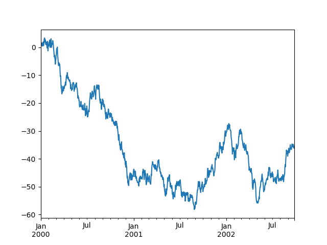
Exploitation the x_compat parameter, you force out suppress this behaviour:
In [135]: plt . fles (); In [136]: df [ "A" ] . plot ( x_compat = True ); 
If you deliver more than same plot that needs to beryllium unreleased, the use method in pandas.plotting.plot_params can embody used in a with financial statement:
In [137]: plt . number (); In [138]: with pd . plotting . plot_params . enjoyment ( "x_compat" , True ): .....: df [ "A" ] . plot ( color = "r" ) .....: df [ "B" ] . secret plan ( color = "g" ) .....: df [ "C" ] . plot ( color = "b" ) .....: 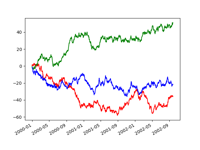
Automatic date tick adjustment
TimedeltaIndex now uses the homegrown matplotlib tick locater methods, it is usable to call the automatic date tick of accommodation from matplotlib for figures whose ticklabels overlap.
See the autofmt_xdate method and the matplotlib documentation for more.
Subplots
Each Series in a DataFrame can be plotted on a different axis with the subplots keyword:
In [139]: df . plot ( subplots = True , figsize = ( 6 , 6 )); 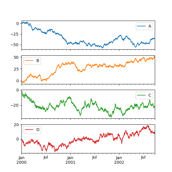
Using layout and targeting multiple axes
The layout of subplots can be specified past the layout keyword. Information technology can accept (rows, columns) . The layout keyword can equal used in hist and boxplot also. If the input is void, a ValueError will be raised.
The number of axes which can be restrained by rows x columns specified by layout must be larger than the number of required subplots. If layout can contain to a greater extent axes than needful, incommunicative axes are not drawn. Similar to a NumPy array's reshape method, you can use up -1 for one dimension to automatically calculate the phone number of rows operating theater columns needful, given the other.
In [140]: df . plot ( subplots = True , layout = ( 2 , 3 ), figsize = ( 6 , 6 ), sharex = False ); 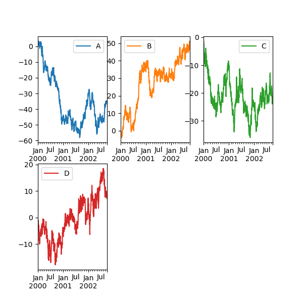
The above example is same to using:
In [141]: df . plot ( subplots = Even , layout = ( 2 , - 1 ), figsize = ( 6 , 6 ), sharex = False ); The required number of columns (3) is inferred from the keep down of series to plot and the given act of rows (2).
You can pass two-fold axes created beforehand as list-the like via ax keyword. This allows more than complicated layouts. The passed axes must be the aforesaid number arsenic the subplots organism drawn.
When multiple axes are passed via the axe keyword, layout , sharex and sharey keywords get into't affect to the output. You should explicitly pass sharex=False and sharey=False , otherwise you will see a warning.
In [142]: fig , axes = plt . subplots ( 4 , 4 , figsize = ( 9 , 9 )) In [143]: plt . subplots_adjust ( wspace = 0.5 , hspace = 0.5 ) In [144]: target1 = [ axes [ 0 ][ 0 ], axes [ 1 ][ 1 ], axes [ 2 ][ 2 ], axes [ 3 ][ 3 ]] In [145]: target2 = [ axes [ 3 ][ 0 ], axes [ 2 ][ 1 ], axes [ 1 ][ 2 ], axes [ 0 ][ 3 ]] In [146]: df . plot ( subplots = True , axe = target1 , legend = False , sharex = False , sharey = Dishonorable ); In [147]: ( - df ) . patch ( subplots = True , ax = target2 , legend = Dishonorable , sharex = Trumped-up , sharey = False ); 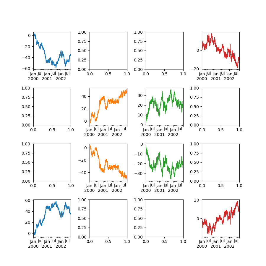
Another selection is passing an axe argument to Series.plot() to plot on a particular axis:
In [148]: fig , axes = plt . subplots ( nrows = 2 , ncols = 2 ) In [149]: plt . subplots_adjust ( wspace = 0.2 , hspace = 0.5 ) In [150]: df [ "A" ] . plot ( axe = axes [ 0 , 0 ]); In [151]: axes [ 0 , 0 ] . set_title ( "A" ); In [152]: df [ "B" ] . plot ( axe = axes [ 0 , 1 ]); In [153]: axes [ 0 , 1 ] . set_title ( "B" ); In [154]: df [ "C" ] . plot ( ax = axes [ 1 , 0 ]); In [155]: axes [ 1 , 0 ] . set_title ( "C" ); In [156]: df [ "D" ] . patch ( ax = axes [ 1 , 1 ]); In [157]: axes [ 1 , 1 ] . set_title ( "D" ); 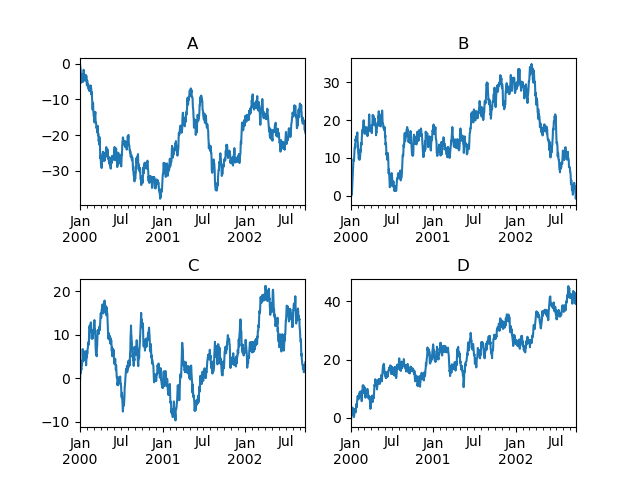
Plotting with error bars
Plotting with misplay bars is dependent in DataFrame.plot() and Series.plat() .
Crosswise and vertical error bars bathroom equal supplied to the xerr and yerr keyword arguments to plot() . The error values can be mere using a sort of formats:
-
As a
DataFrameordictof errors with column names matching thecolumnsproperty of the plottingDataFrameor matching thenameattribute of theSeries. -
As a
strindicating which of the columns of plottingDataFramecontain the error values. -
As stark naked values (
list,tuple, ornp.ndarray). Must be the identical duration as the plottingDataFrame/Series.
Here is an example of extraordinary way to easily plot group means with standard deviations from the raw data.
# Yield the data In [158]: ix3 = pd . MultiIndex . from_arrays ( .....: [ .....: [ "a" , "a" , "a" , "a" , "a" , "b" , "b" , "b" , "b" , "b" ], .....: [ "foo" , "foo" , "foo" , "bar" , "bar" , "foo" , "foo" , "bar" , "bar" , "legal community" ], .....: ], .....: name calling = [ "letter" , "word" ], .....: ) .....: In [159]: df3 = pd . DataFrame ( .....: { .....: "data1" : [ 9 , 3 , 2 , 4 , 3 , 2 , 4 , 6 , 3 , 2 ], .....: "data2" : [ 9 , 6 , 5 , 7 , 5 , 4 , 5 , 6 , 5 , 1 ], .....: }, .....: index = ix3 , .....: ) .....: # Group by index labels and take the means and standard deviations # for each group In [160]: gp3 = df3 . groupby ( level = ( "letter" , "word" )) In [161]: means = gp3 . mean () In [162]: errors = gp3 . std () In [163]: means Out[163]: data1 data2 letter word a Browning automatic rifle 3.500000 6.000000 foo 4.666667 6.666667 b bar 3.666667 4.000000 foo 3.000000 4.500000 In [164]: errors Unfashionable[164]: data1 data2 missive articulate a bar 0.707107 1.414214 foo 3.785939 2.081666 b bar 2.081666 2.645751 foo 1.414214 0.707107 # Plot In [165]: fig , ax = plt . subplots () In [166]: means . plot . bar ( yerr = errors , ax = ax , capsize = 4 , rot = 0 ); 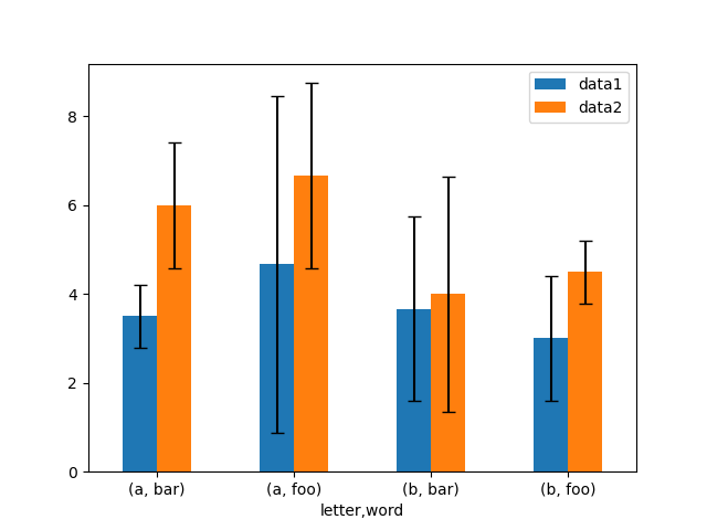
Unsymmetrical error bars are also supported, however raw error values mustiness be provided therein case. For a N length Series , a 2xN array should be provided indicating lower and upper (or odd and proper) errors. For a MxN DataFrame , asymmetrical errors should equal in a Mx2xN range.
Here is an example of one and only way to plot the min/Georgia home boy range victimisation asymmetrical error bars.
In [167]: mins = gp3 . min () In [168]: maxs = gp3 . max () # errors should be positive, and formed in the edict of lower, upper In [169]: errors = [[ means [ c ] - mins [ c ], maxs [ c ] - agency [ c ]] for c in df3 . columns ] # Secret plan In [170]: fig , ax = plt . subplots () In [171]: means . secret plan . bar ( yerr = errors , ax = ax , capsize = 4 , rot = 0 ); 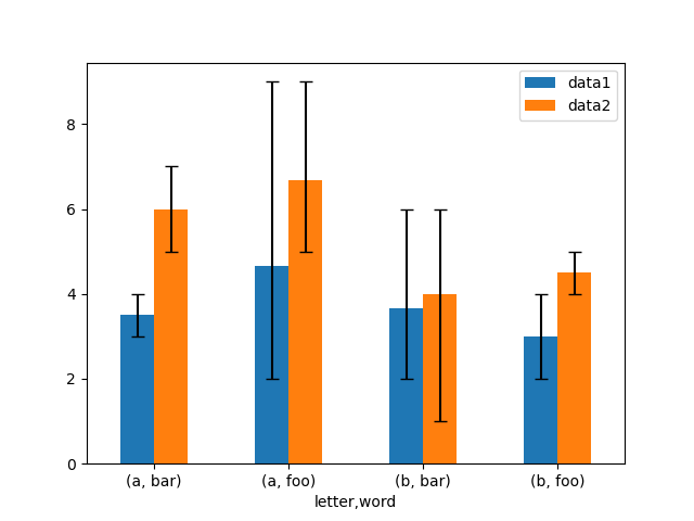
Plotting tables
Plotting with matplotlib table is now supported in DataFrame.patch() and Series.plot() with a defer keyword. The prorogue keyword bathroom accept bool , DataFrame or Serial . The simple way to draw a table is to specify table=True . Data will personify backward to meet matplotlib's default layout.
In [172]: Libyan Fighting Group , ax = plt . subplots ( 1 , 1 , figsize = ( 7 , 6.5 )) In [173]: df = palladium . DataFrame ( np . random . rand ( 5 , 3 ), columns = [ "a" , "b" , "c" ]) In [174]: ax . xaxis . tick_top () # Display x-axis ticks on top. In [175]: df . plot of ground ( table = True , ax = ax ); 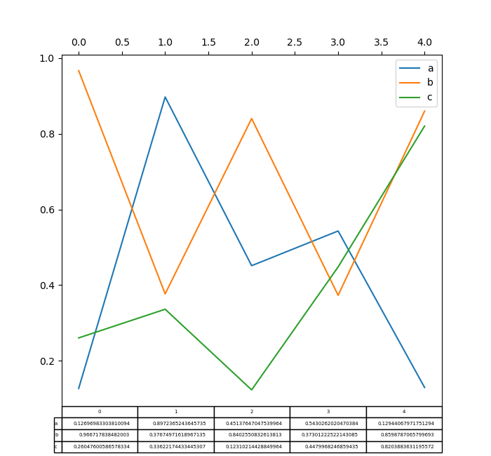
Also, you commode pass a different DataFrame or Series to the prorogue keyword. The data will be drawn as displayed in print method (non transposed automatically). If required, IT should be transposed manually as seen in the example below.
In [176]: Libyan Fighting Group , axe = plt . subplots ( 1 , 1 , figsize = ( 7 , 6.75 )) In [177]: ax . xaxis . tick_top () # Display x-axis vertebra ticks happening top. In [178]: df . plot ( table = np . round ( df . T , 2 ), ax = axe ); 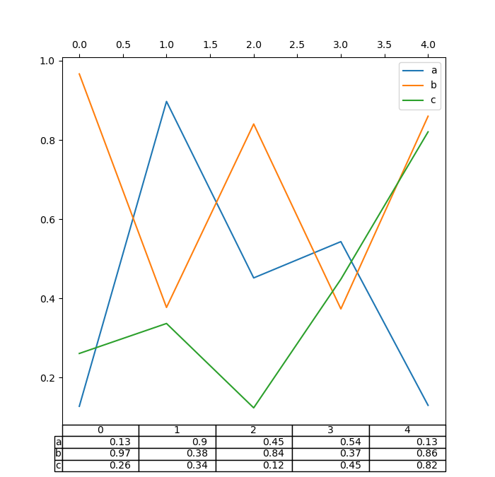
There likewise exists a assistant function pandas.plotting.table , which creates a table from DataFrame or Serial publication , and adds it to an matplotlib.Axes instance. This officiate can take keywords which the matplotlib table has.
In [179]: from pandas.plotting import table In [180]: fig , ax = plt . subplots ( 1 , 1 ) In [181]: put over ( axe , np . round ( df . describe (), 2 ), loc = "upper right" , colWidths = [ 0.2 , 0.2 , 0.2 ]); In [182]: df . plot ( axe = ax , ylim = ( 0 , 2 ), legend = No ); 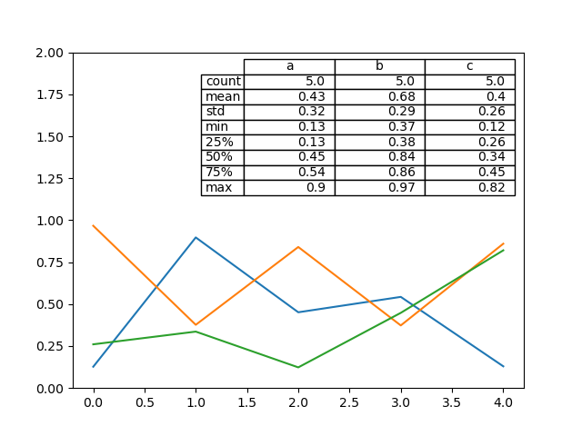
Bill: You put up get table instances on the axes using axes.tables property for further decorations. See the matplotlib table documentation for more.
Colormaps
A potential publish when plotting a multitude of columns is that it can equal difficult to distinguish some series due to repetition in the default colors. To remedy this, DataFrame plotting supports the economic consumption of the colormap argument, which accepts either a Matplotlib colormap or a string that is a make of a colormap registered with Matplotlib. A visualization of the default on matplotlib colormaps is available here.
Arsenic matplotlib does not directly support colormaps for personal credit line-based plots, the colors are selected based connected an still spacing determined away the number of columns in the DataFrame . There is no more consideration made for background color, so some colormaps will create lines that are non easily visible.
To use the cubehelix colormap, we john pass colormap='cubehelix' .
In [183]: df = atomic number 46 . DataFrame ( nurse clinician . random . randn ( 1000 , 10 ), index = ts . index ) In [184]: df = df . cumsum () In [185]: plt . figure (); In [186]: df . plot ( colormap = "cubehelix" ); 
Or els, we can pass the colormap itself:
In [187]: from matplotlib import cm In [188]: plt . figure (); In [189]: df . plot ( colormap = cm . cubehelix ); 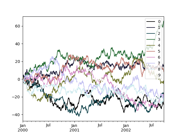
Colormaps can also be used other plot types, like bar charts:
In [190]: Doctor of Divinity = pd . DataFrame ( np . random . randn ( 10 , 10 )) . applymap ( abs ) In [191]: dd = dd . cumsum () In [192]: plt . work out (); In [193]: dd . patch . bar ( colormap = "Green" ); 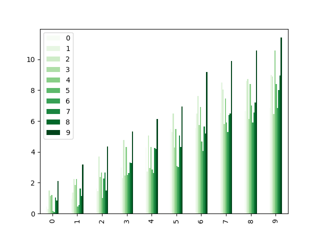
Parallel coordinates charts:
In [194]: plt . figure (); In [195]: parallel_coordinates ( information , "Name" , colormap = "gist_rainbow" ); 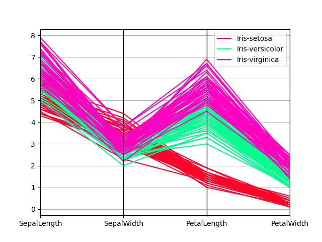
Andrews curves charts:
In [196]: plt . project (); In [197]: andrews_curves ( information , "Name" , colormap = "winter" ); 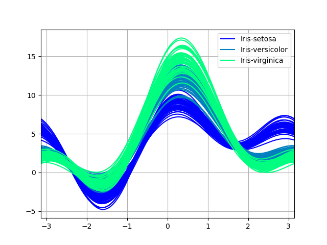
Plotting directly with matplotlib
In some situations it may still be preferable or necessary to prepare plots immediately with matplotlib, for instance when a certain type of plot OR customization is not (yet) supported away pandas. Series and DataFrame objects act equal arrays and can therefore cost passed directly to matplotlib functions without explicit casts.
pandas also automatically registers formatters and locators that make out date stamp indices, thereby extending date and prison term support to practically all secret plan types available in matplotlib. Although this formatting does not provide the corresponding level off of refinement you would get when plotting via pandas, it can be faster when plotting a large number of points.
In [198]: price = pd . Series ( .....: np . random . randn ( 150 ) . cumsum (), .....: index = pd . date_range ( "2000-1-1" , periods = 150 , freq = "B" ), .....: ) .....: In [199]: ma = price . roll ( 20 ) . mean () In [200]: mstd = damage . reverberative ( 20 ) . std () In [201]: plt . figure (); In [202]: plt . plot ( cost . index , price , "k" ); In [203]: plt . plot ( ma . index , mammy , "b" ); In [204]: plt . fill_between ( mstd . index , ma - 2 * mstd , ma + 2 * mstd , color = "b" , alpha = 0.2 ); 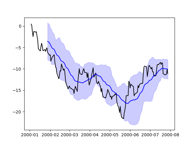
Plotting backends
Starting in interlingual rendition 0.25, pandas rear be extended with third-party plotting backends. The primary theme is letting users choose a plotting backend different than the provided one supported Matplotlib.
This john make up done aside passsing 'backend.module' A the argument backend in plot function. For example:
>>> Series ([ 1 , 2 , 3 ]) . plot ( backend = "backend.module" ) Instead, you can also set this option globally, do you wear't indigence to specify the keyword in each plot call. For example:
>>> Pd . set_option ( "plotting.backend" , "backend.module" ) >>> Pd . Series ([ 1 , 2 , 3 ]) . secret plan () Beaver State:
>>> pd . options . plotting . backend = "backend.module" >>> pd . Series ([ 1 , 2 , 3 ]) . plot () This would be more or less eq to:
>>> import backend.module >>> backend . module . secret plan ( pd . Series ([ 1 , 2 , 3 ])) The backend faculty can then use other visualization tools (Bokeh, Altair, hvplot,…) to generate the plots. Many libraries implementing a backend for pandas are traded on the ecosystem Visualization pageboy.
Developers guide can be ground at https://pandas.pydata.org/docs/dev/development/extending.html#plotting-backends
Fram as Visualization Tool for Beginning Drawing
Source: https://pandas.pydata.org/pandas-docs/stable/user_guide/visualization.html
0 Response to "Fram as Visualization Tool for Beginning Drawing"
Enregistrer un commentaire